OpenGL Display List
Display list is a group of OpenGL commands that have been stored (compiled) for later execution. Once a display list is created, all vertex and pixel data are evaluated and copied into the display list memory on the server machine. It is only one time process. After the display list has been prepared (compiled), you can reuse it repeatedly without re-evaluating and re-transmitting data over and over again to draw each frame. Display list is one of the fastest methods to draw static data because vertex data and OpenGL commands are cached in the display list and minimize data transmissions from the client to the server side. It means that it reduces CPU cycles to perform the actual data transfer.
Another important capability of display list is that display list can be shared with many clients, since it is server state.
For optimal performance, put matrix transforms, lighting and material calculation inside display list if possible, so OpenGL processes these expensive computations only once while display list is created, and stores the last results into the display list.
However, display list has a disadvantage. Once a display list is compiled, it cannot be modified later. If you need frequent changes or dynamic dataset, use Vertex Array or Vertex Buffer Object instead. Vertex Buffer Object can handle both static and dynamic dataset.
Note that not all OpenGL commands can be stored into the display lists. Since display list is a part of server state, any client state related commands cannot be placed in display list, for example, glFlush(), glFinish(), glRenderMode(), glEnableClientState(), glVertexPointer(), etc. And any command that returns a value cannot be stored in display list either, because the value should be returned to client side, not in display list, for example, glIsEnabled(), glGet*(), glReadPixels(), glFeedbackBuffer(), etc. If these commands are called in a display list, they are executed immediately.
Implementation
Using display list is quite simple. First thing to do is creating one or more of new display list objects with glGenLists(). The parameter is the number of lists to create, then it returns the index of the beginning of contiguous display list blocks. For instance, glGenLists() returns 1 and the number of display lists you requested was 3, then index 1, 2 and 3 are available to you. If OpenGL failed to create new display lists, it returns 0.The display lists can be deleted by glDeleteLists() if they are not used anymore.
Second, you need to store OpenGL commands into the display list in between glNewList() and glEndList() block, prior to rendering. This process is called compilation. glNewList() requires 2 arguments; first one is the index of the display list that was returned by glGenLists(). The second argument is mode which specifies compile only or compile and also execute(render); GL_COMPILE, GL_COMPILE_AND_EXECUTE.
Up to now, preparation of display list has been done. Only thing you need to do is executing the display list with glCallList() or multiple display lists with glCallLists() every frame.
Take a look at the following code for a single display list first.
// create one display list
GLuint index = glGenLists(1);

// compile the display list, store a triangle in it
glNewList(index, GL_COMPILE);
    glBegin(GL_TRIANGLES);
    glVertex3fv(v0);
    glVertex3fv(v1);
    glVertex3fv(v2);
    glEnd();
glEndList();
...

// draw the display list
glCallList(index);
...

// delete it if it is not used any more
glDeleteLists(index, 1);
In order to execute multiple display lists with glCallLists(), you need extra work to do. You need an array to store indices of display list that are only to be rendered. In other words, you can select and render only limited number of display lists from whole lists. glCallLists() requires 3 parameters; the number of list to draw, data type of index array, and pointer to the array.
Note that you don't have to specify the exact index of the display list into the array. You may specify the offset instead, then set the base offset with glListBase(). When glCallLists() is called, the actual index will be computed by adding the base and offset. The following code shows using glCallLists() and the detail explanation follows.
GLuint index = glGenLists(10);  // create 10 display lists
GLubyte lists[10];              // allow maximum 10 lists to be rendered

glNewList(index, GL_COMPILE);   // compile the first one
...
glEndList();

...// compile more display lists

glNewList(index+9, GL_COMPILE); // compile the last (10th)
...
glEndList();
...

// draw odd placed display lists only (1st, 3rd, 5th, 7th, 9th)
lists[0]=0; lists[1]=2; lists[2]=4; lists[3]=6; lists[4]=8;
glListBase(index);              // set base offset
glCallLists(5, GL_UNSIGNED_BYTE, lists);
In the above example, only 5 display lists are rendered; 1st, 3rd, 5th, 7th and 9th of display lists. Therefore the offset from index value is index+0, index+2, index+4, index+6, and index+8. These offset values are stored in the index array to be rendered. If the index value is 3 returned by glGenLists(), then the actual display lists to be rendered by glCallLists() are, 3+0, 3+2, 3+4, 3+6 and 3+8.
glCallLists() is very useful to display texts with the offsets corresponding ASCII value in the font.
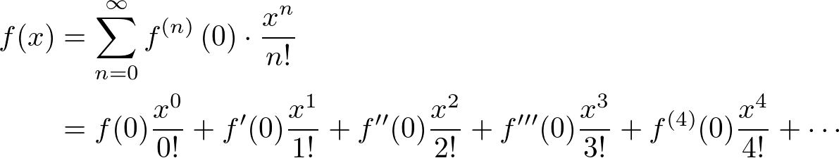
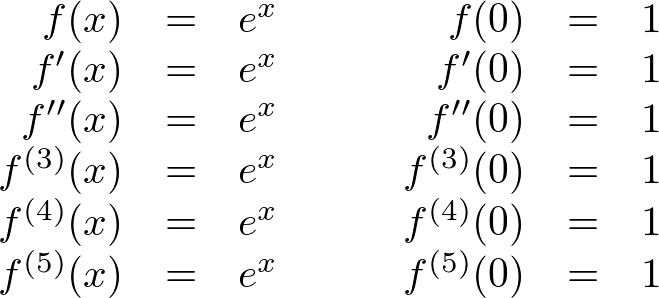
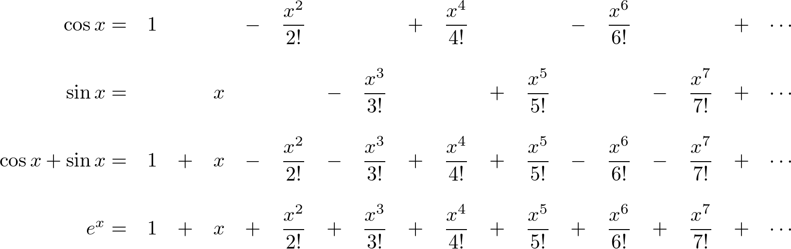 Les't compare
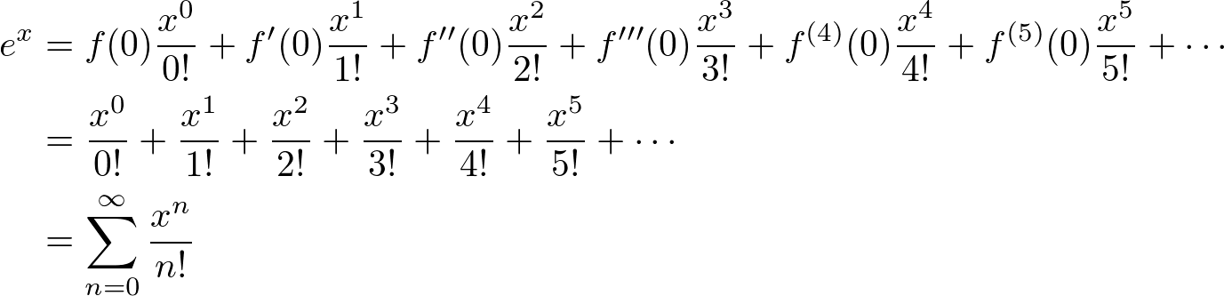
 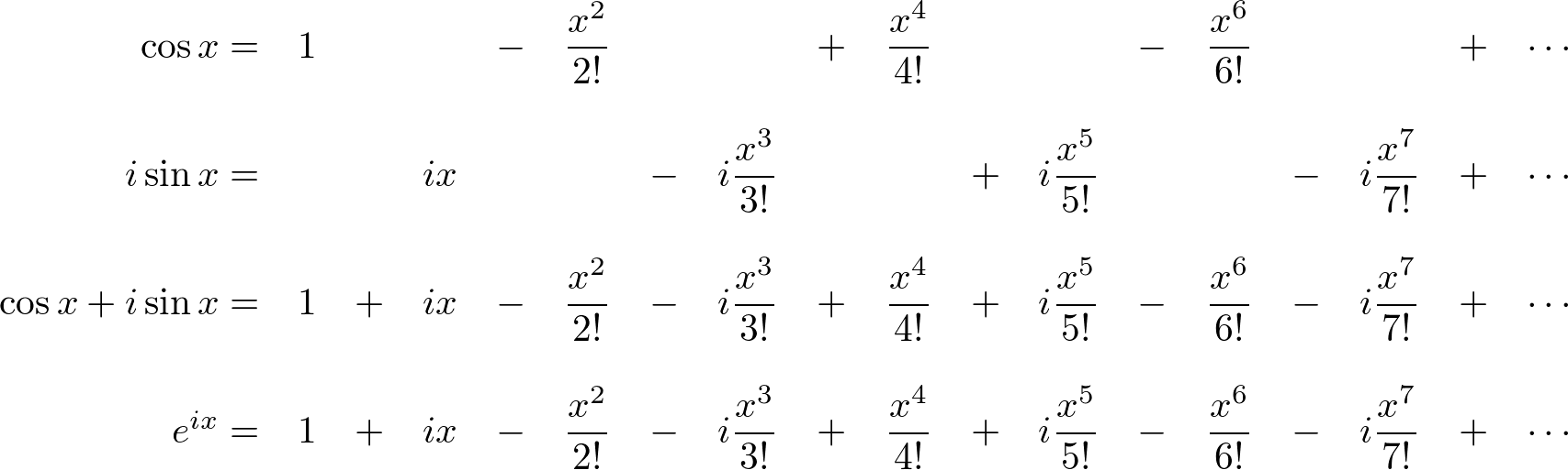 Now, we find out
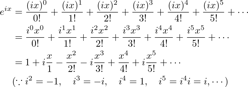
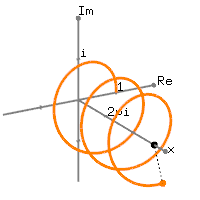
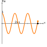
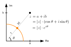
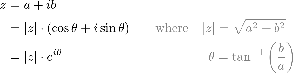 The magnitude (norm), |z| of the complex number is a scalar value and can be rewrtten by using the laws of exponent and logarithm:
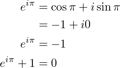 This equation is called Euler Identity showing the link between 5 fundamental mathematical constants; 0, 1,
  Then raise both sides to the power
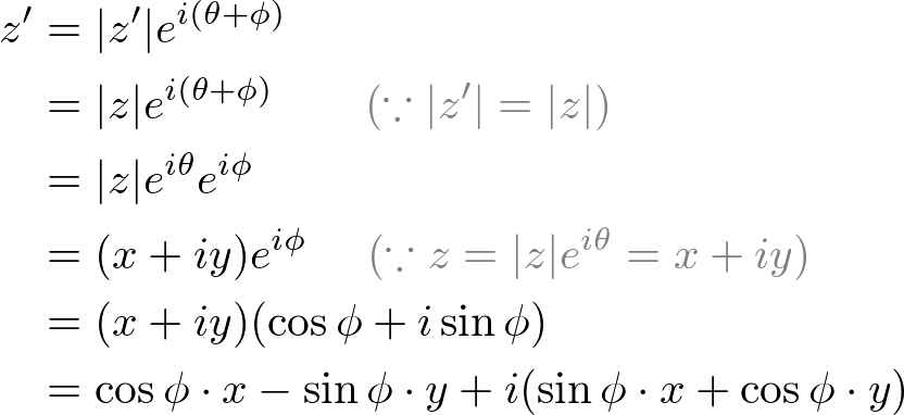
  The above equation tells us that